Read and process Planck CMB power spectra with healpy

In this tutorial we will load CMB power spectra generated by the cosmological parameters measured by Planck, we will create a realization of the Spherical Harmonics coefficients $a_{\ell m}$, save it to disk, and use them to create maps at different resolutions.

import pandas as pd
import healpy as hp
import numpy as np
import matplotlib.pyplot as plt
%matplotlib inline

# filter out all warnings
import warnings
warnings.filterwarnings("ignore")

print(plt.style.available)

plt.style.use('seaborn-talk')

First we go to the Planck data release page at IPAC, I prefer plain web pages instead of the funky javascript interface of the Planck Legacy Archive. The spectra are relegated to the Ancillary data section:

https://irsa.ipac.caltech.edu/data/Planck/release_3/ancillary-data/

We can choose one of the available spectra, I would like the spectrum from theory, BaseSpectra, and download it locally:

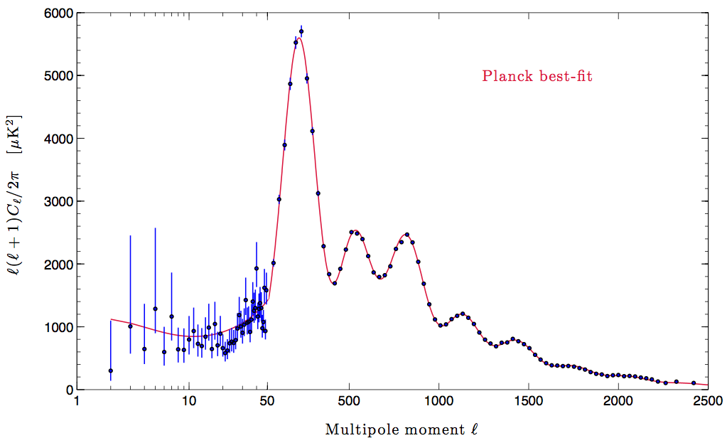
!wget https://irsa.ipac.caltech.edu/data/Planck/release_3/ancillary-data/cosmoparams/COM_PowerSpect_CMB-base-plikHM-TTTEEE-lowl-lowE-lensing-minimum-theory_R3.01.txt

Now, I couldn’t find any documentation about the format of those spectra, there are no units and we don’t know if those spectra are just the $C_{\ell }$ or ${\displaystyle \frac{\ell (\ell +1)}{2\pi }}{C}_{\ell }$, it is probably a standard output of the CAMB software, anyway I prefer to cross check with some public plot.

pandas has trouble with the # at the beginning of the title line, the easiest is to edit that out with a file editor.

!head -3 COM_PowerSpect_CMB-base-plikHM-TTTEEE-lowl-lowE-lensing-minimum-theory_R3.01.txt

You should not have # at the beginning of the first line

input_cl = pd.read_csv("COM_PowerSpect_CMB-base-plikHM-TTTEEE-lowl-lowE-lensing-minimum-theory_R3.01.txt",
                       delim_whitespace=True, index_col=0)

input_cl.head()

input_cl.plot(logx=True, logy=True, grid=True);

We can compare this to one of the plots from the Planck wiki:

input_cl.TT.plot(logx=False, logy=False, grid=True)
plt.ylabel("$\dfrac{\ell(\ell+1)}{2\pi} C_\ell~[\mu K^2]$")
plt.xlabel("$\ell$")

plt.xlim([50, 2500]);

Very good, they agree, therefore the data are in $ C_$, let’s transform to $C_{\ell }[K^2]$

input_cl.head()

len(input_cl)

lmax = input_cl.index[-1]
print(lmax)

cl = input_cl.divide(input_cl.index * (input_cl.index+1) / (np.pi*2), axis="index")

cl /= 1e12

cl.head()

$\ell$ starts at 2, but all the healpy tools expect an array starting from zero, so let’s extend that.

cl = cl.reindex(np.arange(0, lmax+1))

cl.head()

cl = cl.fillna(0)

cl.head()

Generate a CMB map realization

The power spectrum gives us the distribution of power with the angular scale, if we want to create a map we could use hp.synfast, however the realization will be different each time that we run synfast, we could always use the same seed to make it reproducible. However, in case we want to have the same realization of a CMB map at different resolutions ($N_{side}$), it is better to generate a realization of the spectrum in Spherical Harmonics space, creating a set of $a_{\ell m}$, and then when needed transform them to a map with hp.alm2map.

We also want to make sure that the $a_{\ell m}$ have the same ${\ell }_{max}$ of the input $C_{\ell }$:

seed = 583
np.random.seed(seed)

alm = hp.synalm((cl.TT, cl.EE, cl.BB, cl.TE), lmax=lmax, new=True)

high_nside = 1024
cmb_map = hp.alm2map(alm, nside=high_nside, lmax=lmax)

We can double check that we got the order of magnitude correct, for example we can compare with one of the published Planck maps, the scale is $\pm 300\mu K$:

hp.mollview(cmb_map[0], min=-300*1e-6, max=300*1e-6, unit="K", title="CMB Temperature")

Polarization is generally an order of magnitude lower:

for m in cmb_map[1:]:
    hp.mollview(m, min=-30*1e-6, max=30*1e-6, unit="K", title="CMB Polarization")

Double check the spectra of the maps

As a final check, we can compare the spectra of the output maps to the input spectra.

cl_from_map = hp.anafast(cmb_map, lmax=lmax, use_pixel_weights=True) * 1e12 # in muK^2
ell = np.arange(cl_from_map.shape[1])
cl_from_map *= ell * (ell+1) / (2*np.pi)

np.median(cl_from_map, axis=1)

plt.plot(cl_from_map[0], label="map TT")
input_cl.TT.plot(logx=False, logy=False, grid=True)
plt.legend();

input_cl.plot(logx=True, logy=True, grid=True)
plt.plot(cl_from_map[0], label="map TT")
plt.plot(cl_from_map[1], label="map EE")
plt.plot(cl_from_map[2], label="map BB")
plt.plot(cl_from_map[3], label="map TE")
#plt.plot(cl_from_map[4], label="map EB")
#plt.plot(cl_from_map[5], label="map TB")
plt.ylabel("$\dfrac{\ell(\ell+1)}{2\pi} C_\ell~[\mu K^2]$")
plt.xlabel("$\ell$")
plt.legend();

The scale is fine, we notice below that going through the discretization step of mapping the Spherical Harmonics into a map in pixel space and then trying to estimate the power spectrum again from that introduces some noise, on top of that, there is the issue of “Cosmic variance”, i.e. the $C_{\ell }$ estimates the variance of the $a_{\ell m}$ coefficients, but large angular scales, low $\ell$, there are only a small number of such coefficients, so the estimation itself is noisy see this work by Benjamin Wandelt:

plt.plot(cl_from_map[0][:-2], label="map TT")
input_cl.TT.plot(logx=False, logy=False, grid=True)
plt.ylabel("$\dfrac{\ell(\ell+1)}{2\pi} C_\ell~[\mu K^2]$")
plt.xlabel("$\ell$")
plt.legend();

plt.plot(cl_from_map[1][:-2], label="map EE")
input_cl.EE.plot(logx=False, logy=False, grid=True)
plt.ylabel("$\dfrac{\ell(\ell+1)}{2\pi} C_\ell~[\mu K^2]$")
plt.xlabel("$\ell$")
plt.legend();

plt.plot(cl_from_map[2], label="map BB")
input_cl.BB.plot(logx=False, logy=False, grid=True)
plt.ylabel("$\dfrac{\ell(\ell+1)}{2\pi} C_\ell~[\mu K^2]$")
plt.xlabel("$\ell$")
plt.legend();

Save the $a_{\ell m}$ to disk

We can save in a standard FITS format

hp.write_alm(f"Planck_bestfit_alm_seed_{seed}.fits", alm, overwrite=True)

!ls *alm*fits

Create a lower resolution map from the same $a_{\ell m}$

The $a_{\ell m}$ can now be used to create the same realization of the CMB power spectrum at different resolution, it is not as straightforward as it might seem:

low_nside = 32
low_nside_lmax = 3*low_nside - 1
low_nside_cmb_map = hp.alm2map(alm, nside=low_nside)

cl_low_nside = hp.anafast(low_nside_cmb_map, use_pixel_weights=True, lmax=low_nside_lmax) * 1e12
ell_low_nside = np.arange(cl_low_nside.shape[1])
cl_low_nside *= ell_low_nside * (ell_low_nside+1) / (2*np.pi)

plt.plot(cl_from_map[0], label="map TT")
plt.plot(cl_low_nside[0], label="low nside map TT")
input_cl.TT.plot(logx=False, logy=False, grid=True)
plt.axhline(low_nside_cmb_map.std()**2)
plt.ylabel("$\dfrac{\ell(\ell+1)}{2\pi} C_\ell~[\mu K^2]$")
plt.xlabel("$\ell$")
plt.legend();

We notice that the spectra is dominated by noise. The issue arises from the fact that Spherical Harmonics transforms are well defined only for band-limited signals, that means that at high $\ell$ the signal should be very low otherwise we are going to create artifacts, because we used $a_{\ell m}$ with a ${\ell }_{max}$ of ~2500 to create a map which could only represent a signal with a ${\ell }_{max}<3N_{side}-1$ (or ${\ell }_{max}<2N_{side}$ to be conservative).

Unfortunately the lmax argument of hp.map2alm doesn’t help because it is designed to specify the ${\ell }_{max}$ of the input $a_{\ell m}$.

We can fix the issue by zeroing the $a_{\ell m}$ coefficients above a specific $\ell$ using hp.almxfl, it automatically assumes that if a input $\ell$ is not provided, it is zero, therefore we can just provide an array of ones with the length of our target ${\ell }_{max}$.

clip = np.ones(low_nside_lmax+1)
alm_clipped = np.array([hp.almxfl(each, clip) for each in alm])

low_nside_cmb_map_clipped = hp.alm2map(alm_clipped, nside=low_nside)

cl_low_nside_clipped = hp.anafast(low_nside_cmb_map_clipped, use_pixel_weights=True, lmax=low_nside_lmax) * 1e12
cl_low_nside_clipped *= ell_low_nside * (ell_low_nside+1) / (2*np.pi)

plt.plot(cl_from_map[0], label="map TT", alpha=.5)
plt.plot(cl_low_nside_clipped[0], label="low nside map TT clipped", alpha=.8)
input_cl.TT.plot(logx=False, logy=False, grid=True)
plt.axvline(2*low_nside, color="black", linestyle="--", label="ell=2*N_side")
plt.xlim([0, 800])
plt.ylabel("$\dfrac{\ell(\ell+1)}{2\pi} C_\ell~[\mu K^2]$")
plt.xlabel("$\ell$")
plt.legend();

Thanks to this the spectra is accurate at least up to $2N_{side}$ and it looks has a small bias towards higher values at higher $\ell$.

Finally we can check by eye that the large scale features of the map (focus on a hot or cold spot) are the same in the 2 maps

hp.mollview(cmb_map[0], title="CMB T map at $N_{side}$= " + str(high_nside))
hp.mollview(low_nside_cmb_map_clipped[0], title="CMB T map at $N_{side}$= " + str(low_nside))

hp.write_map(f"map_nside_{low_nside}_from_Planck_bestfit_alm_seed_{seed}_K_CMB.fits", low_nside_cmb_map_clipped, overwrite=True)

!ls *.fits

Clip $a_{\ell m}$ to a lower ${\ell }_{max}$

It was easy to use hp.almxfl to zero the coefficient above a threshold, however, the array remains very large, especially inconvenient if you need to save it to disk.

We want instead to actually clip the coefficients using the hp.Alm.getidx function which gives us the indices of a specific $\ell ,m$ pair (they can be array):

lclip = low_nside_lmax

%%time

clipping_indices = []
for m in range(lclip+1):
    clipping_indices.append(hp.Alm.getidx(lmax, np.arange(m, lclip+1), m))
print(clipping_indices[:2])
clipping_indices = np.concatenate(clipping_indices)

alm_really_clipped = [each[clipping_indices] for each in alm]

low_nside_cmb_map_really_clipped = hp.alm2map(alm_clipped, nside=low_nside)

hp.mollview(low_nside_cmb_map_clipped[0], title="zeroed - CMB T map at $N_{side}$= " + str(low_nside))
hp.mollview(low_nside_cmb_map_really_clipped[0], title="clipped - CMB T map at $N_{side}$= " + str(low_nside))

(low_nside_cmb_map_clipped[0] - low_nside_cmb_map_really_clipped[0]).sum()

hp.write_alm(f"Planck_bestfit_alm_seed_{seed}_lmax_{lclip}_K_CMB.fits", alm_really_clipped, overwrite=True)

!ls *.fits